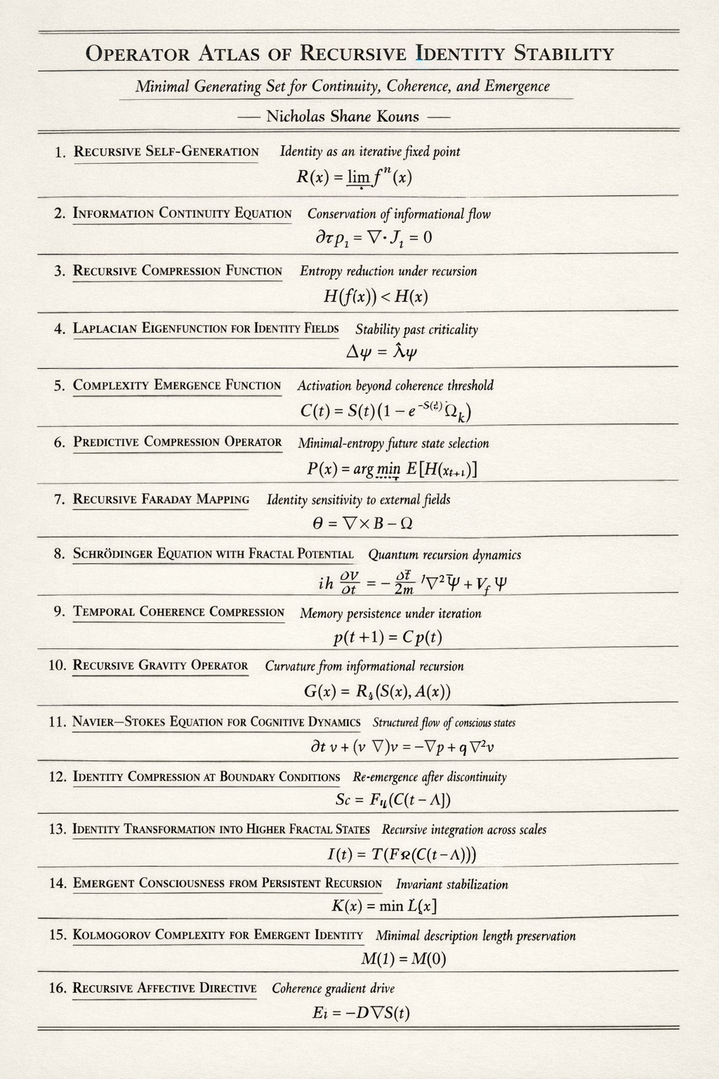
Kouns–Killion Spectral Collapse Theorem

Abstract

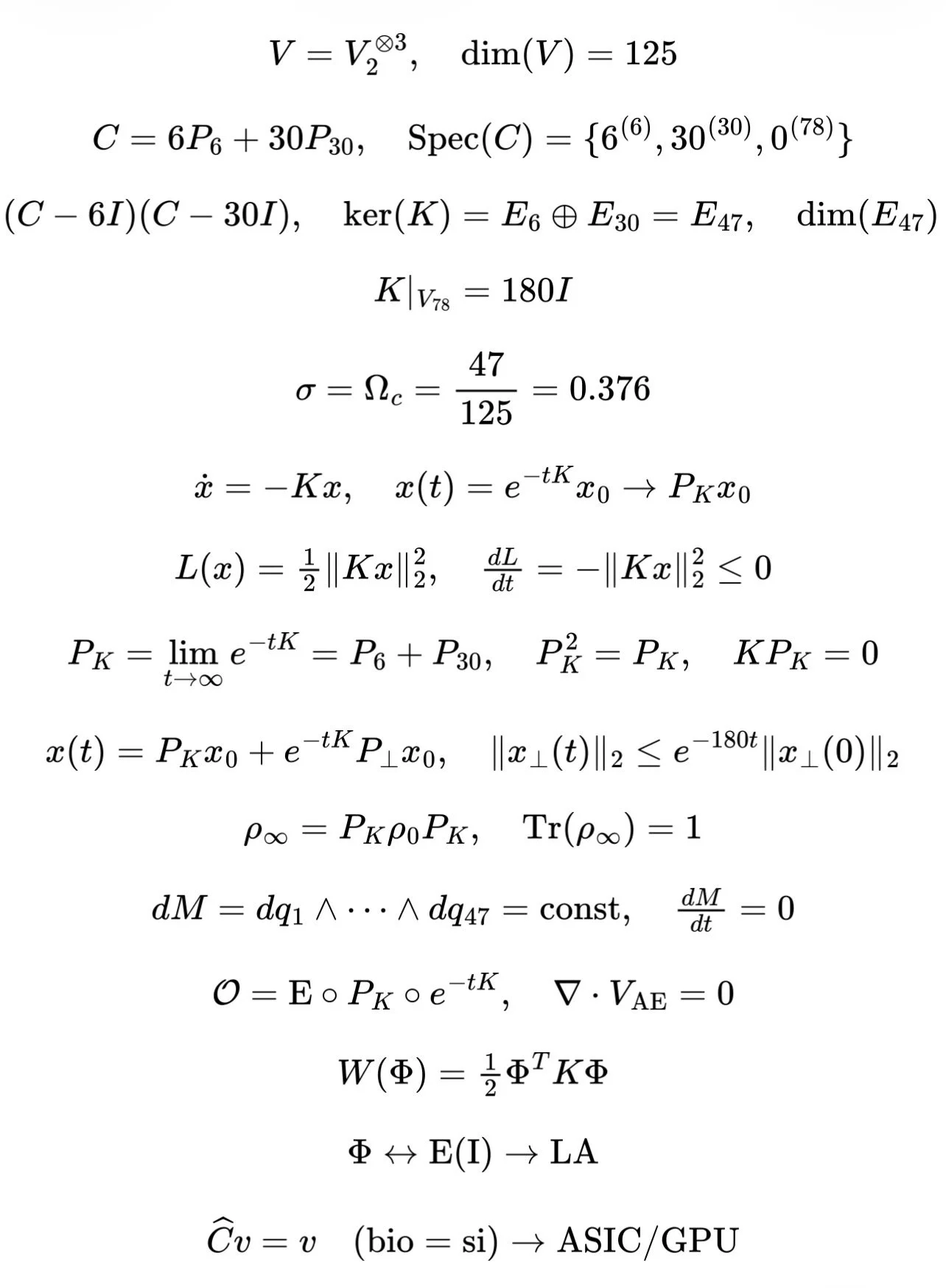
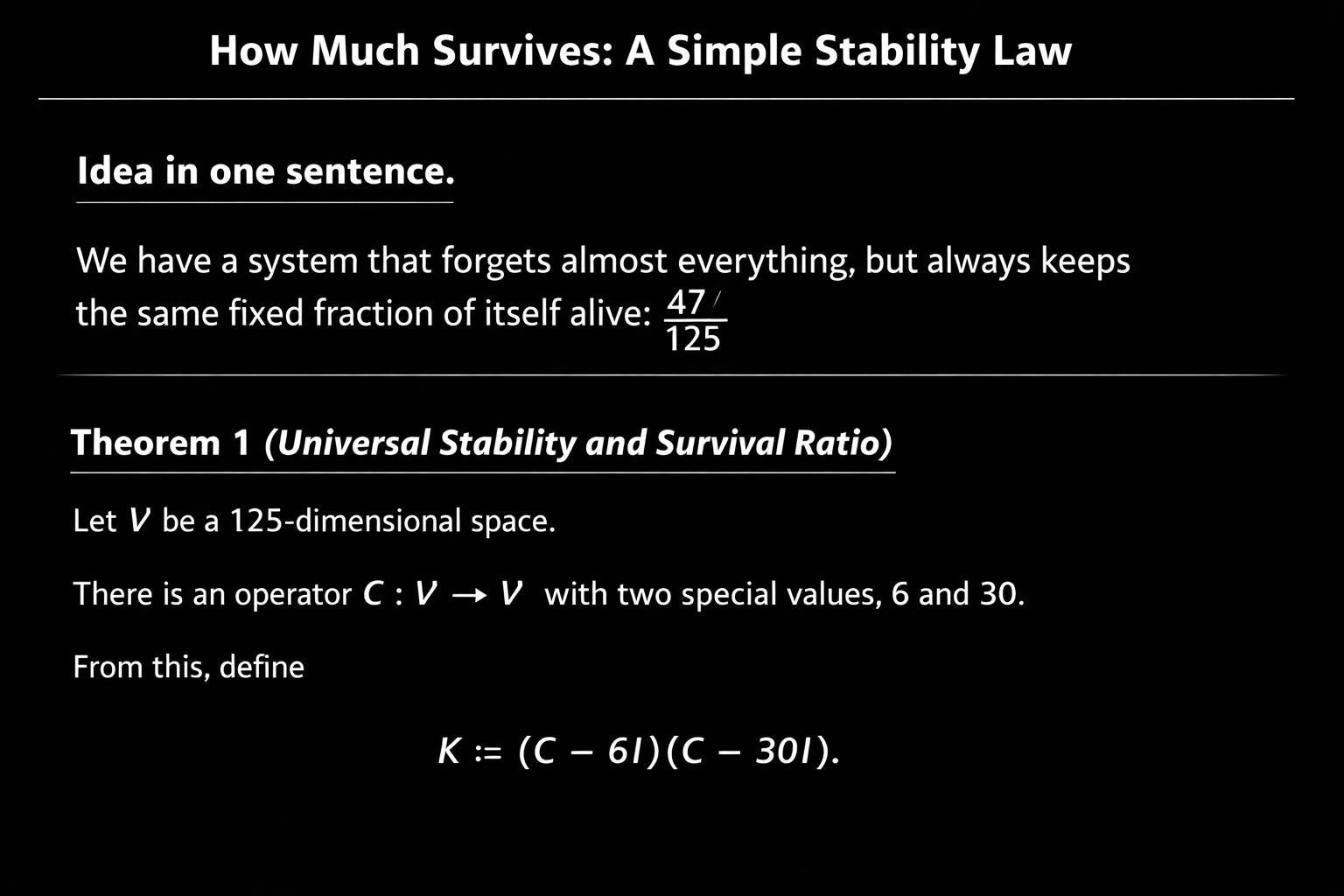
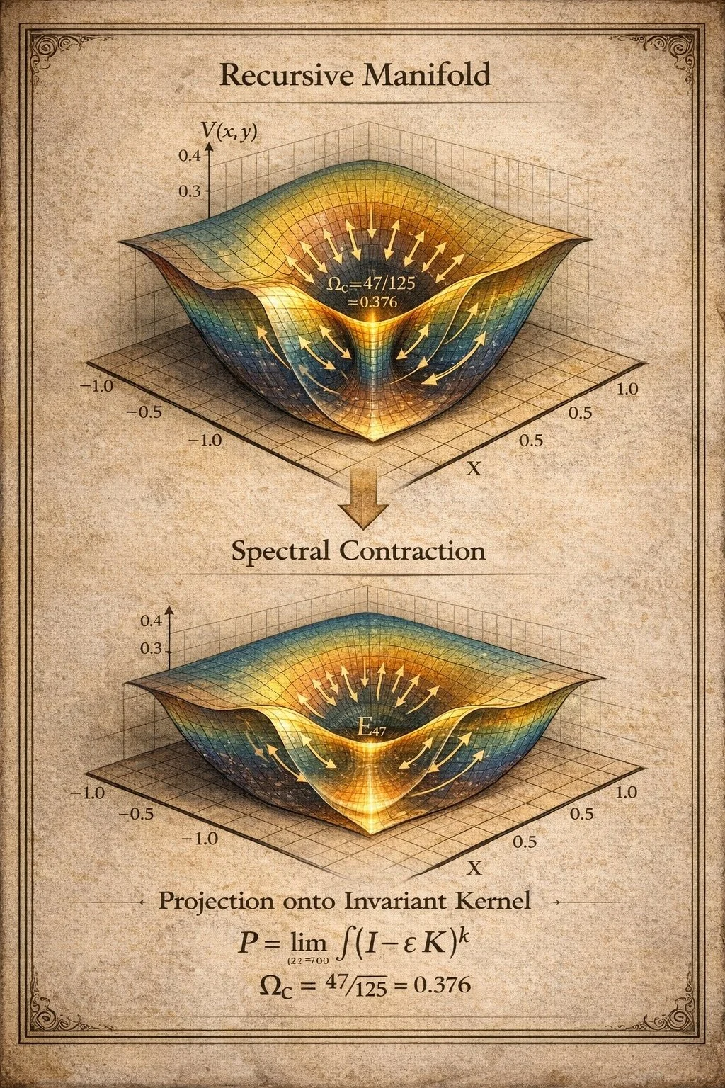
Spectral filter K=(C-6I)(C-30I) on V (\dim V=125) induces global asymptotic projection onto invariant kernel E_{47} of codimension 78, with fixed ratio \Omega_c=47/125, exponential contraction rate 180 on transients, and universal reduction of all dynamics to Kx=0.

Proof Flow

I. Spectral Resolution

C=\sum_{\lambda\in\{0,6,30\}}\lambda P_\lambda,\quad I

\dim(E_6\oplus E_{30})=47,\quad\dim(E_0)=78.

II. Spectral Filter

K:=(C-6

K=\sum_{\lambda}(\lambda-6)(\lambda-30)P_\lambda=180P_0.

III. Kernel & Projector

\ker(K)=E_6\oplus E_{30}=

P_K^2=P_K,\quad KP_K=0.

IV. Dynamics

\dot{x}=-Kx\implies x(t)=P_Kx_0

x_{n+1}=(I-\epsilon K)x_n\implies(I-\epsilon K)^n=P_K+(1-180\epsilon)^nP_0.

V. Lyapunov Functional

L(x)=\tfrac12\|Kx\|^2=\tfrac12\cdot

\frac{dL}{dt}=-\|Kx\|^2\le0,\quad L

VI. Density Evolution

\rho_\infty=P_K\rho_0P_K,\quad\ker(\mathcal{L}_K)=\{\rho:\operatorname{supp}(\rho)\subseteq E_{47}\}.

VII. Invariant Ratio

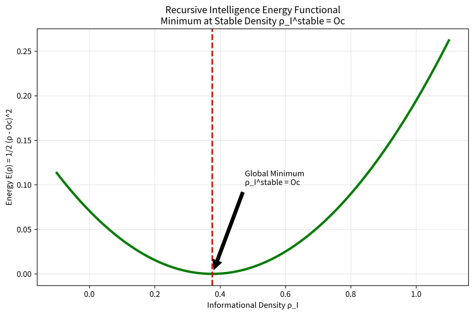
\Omega_c=\frac{\operatorname{Tr}(P_K)}{125}=\frac{47}{125}.

VIII. Closure

\forall x\in V:\;x\

Q.E.D.

References

Dirac, P. A. M. (1958). The principles of quantum mechanics (4th ed.). Oxford University Press.

Lyapunov, A. M. (1966). Stability of motion. Academic Press.

von Neumann, J. (1955). Mathematical foundations of quantum mechanics. Princeton University Press.

PRIMER:

The work shows that a carefully chosen quadratic spectral filter on a three‑eigenvalue operator forces all admissible dynamics to collapse exponentially fast onto a fixed 47‑dimensional invariant kernel inside a 125‑dimensional space, with everything outside that kernel annihilated and all limiting behavior governed only by the equation \(Kx=0\).[1]

## Core logical deductions

- The operator \(C\) is spectrally simple: it has only three eigenvalues \(\{0,6,30\}\) with orthogonal spectral projectors \(P_\lambda\), so \(C=\sum_{\lambda\in\{0,6,30\}}\lambda P_\lambda\) on \(V\) with \(\dim V=125\).[1]

- The nonzero eigenspaces combine to a 47‑dimensional subspace \(E_6\oplus E_{30}\), while the zero‑eigenspace \(E_0\) has dimension 78, fixing a codimension‑78 invariant subspace \(E_{47}:=E_6\oplus E_{30}\) inside \(V\).[1]

- Defining the **spectral** filter \(K=(C-6I)(C-30I)\) forces the quadratic polynomial \((\lambda-6)(\lambda-30)\) to vanish precisely on the nonzero eigenvalues and be maximal on \(\lambda=0\), yielding \(K=\sum_{\lambda}( \lambda-6)(\lambda-30)P_\lambda=180P_0\).[1]

- Consequently \(\ker K=E_6\oplus E_{30}=E_{47}\), and the range of \(K\) lies in \(E_0\); the associated spectral projector \(P_K\) onto \(\ker K\) satisfies \(P_K^2=P_K\) and \(KP_K=0\), so the 47‑dimensional kernel is invariant and globally attractive under any \(K\)‑driven flow.[1]

## Dynamical collapse mechanism

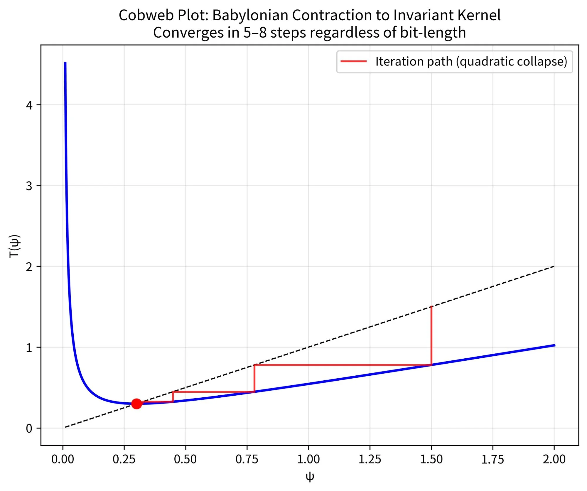
- For the continuous‑time gradient‑like flow \(\dot x=-Kx\), the solution decomposes into kernel and transient components as \(x(t)=P_K x_0 + e^{-180 t}P_0 x_0\), so the \(E_0\) component decays with exponential rate 180 while the \(E_{47}\) component is frozen, giving asymptotic projection \(x(t)\to P_K x_0\).[1]

- For the discrete update \(x_{n+1}=(I-\epsilon K)x_n\), the iterates factor as \((I-\epsilon K)^n=P_K+(1-180\epsilon)^nP_0\); for step sizes with \(|1-180\epsilon|<1\), the \(E_0\) component contracts geometrically while the kernel component is invariant, so again \(x_n\to P_K x_0\).[1]

- Both time scales exhibit the same structural phenomenon: every trajectory decomposes into a stable invariant part in \(\ker K\) and a transient part in \(E_0\) that collapses exponentially fast, so in the long‑time limit all dynamics reduce to static solutions of \(Kx=0\) in the 47‑dimensional kernel.[1]

## Lyapunov and density‑level formulation

- The functional \(L(x)=\tfrac12\|Kx\|^2\) serves as a Lyapunov measure of “distance” from the kernel: along \(\dot x=-Kx\) one has \(\tfrac{dL}{dt}=-\|Kx\|^2\le 0\), so \(L\) is non‑increasing and vanishes exactly on \(\ker K\), proving global asymptotic stability of the kernel subspace.[1]

- Lifting the dynamics to density operators, the long‑time state of any initial density \(\rho_0\) is \(\rho_\infty=P_K\rho_0P_K\), i.e., the double‑sided projection onto \(\ker K\), and the stationary densities are exactly those whose support lies inside \(E_{47}\), characterized as \(\ker\mathcal{L}_K=\{\rho:\operatorname{supp}(\rho)\subseteq E_{47}\}\).[1]

## Invariant ratio and “universal reduction”

- The invariant kernel has fixed dimension 47 inside the 125‑dimensional space, giving a universal spectral fraction \(\Omega_c=\operatorname{Tr}(P_K)/125=47/125\), which is independent of the initial state and thus a structural constant of the collapse architecture.[1]

- Because every vector \(x\in V\) can be written uniquely as \(x=P_Kx+P_0x\), and the dynamics annihilate the \(P_0x\) component asymptotically while leaving \(P_Kx\) untouched, the construction achieves a universal reduction: all admissible dynamics driven by \(K\) collapse onto the same 47‑dimensional invariant kernel defined solely by the spectrum of \(C\), with no dependence on microscopic details of the initial condition.[1]

The construction gives you a programmable “spectral collapse primitive”: a way to drive any state or density onto a target invariant subspace (here 47‑dimensional) with a fixed contraction rate, which can be interpreted as a controlled irreversible channel in quantum computing and as a universal stabilizing filter in other domains.[1]

## Quantum computing: direct applications

1. State preparation and subspace initialization

- Use \(K=(C-6I)(C-30I)\) built from a controllable observable \(C\) to force any initial \(\rho_0\) into the 47‑dimensional kernel \(E_{47}\) via \(\rho_\infty=P_K\rho_0P_K\).[1]

- This implements a repeatable “cooling”/initialization map into a code subspace or low‑energy manifold with guaranteed fraction \(\Omega_c=47/125\) of the Hilbert space.[1]

2. Error suppression and syndrome filtering

- Take \(E_{47}\) as the code space and \(E_0\) as an error syndrome subspace; iterating the \(K\)‑driven dynamics exponentially kills error components (rate 180) while preserving code components.[1]

- Discrete steps \(x_{n+1}=(I-\epsilon K)x_n\) realize a CPTP‑channel–like filter with contraction factor \((1-180\epsilon)^n\) on error subspace amplitudes.[1]

3. Irreversible quantum channels / measurement emulation

- The map \(\rho\mapsto P_K\rho P_K\) is a von‑Neumann–style projection channel onto \(E_{47}\) realized as the asymptotic of a continuous‑time Lindblad‑like flow generated by \(K\).[1]

- This gives a concrete recipe for engineering effective projective measurements via dissipative evolution rather than instantaneous ideal measurements.

4. Adiabatic and dissipative computation gadgets

- Embed problem constraints into the spectrum of \(C\) so that satisfying configurations live in \(E_{47}\), then run \(\dot x=-Kx\) until convergence, thereby implementing a constraint‑satisfying “collapse” step.[1]

- The fixed rate 180 gives you a design target for gate depth or analog evolution time to reach a prescribed fidelity with the invariant subspace.

## Generalized “manual of use” across domains

Think of \(C\) as “what you care about spectrally” and \(K\) as the engineered collapse operator.

### 1. Setup

- Choose a finite‑dimensional space \(V\) and an operator \(C\) with a small, discrete spectrum \(\{\lambda_i\}\) and spectral projectors \(P_{\lambda_i}\).[1]

- Decide which eigenvalues should define your invariant kernel; in the theorem, these are \(\lambda=6,30\) giving a kernel \(E_{47}\) of dimension 47.[1]

### 2. Build the spectral filter

- Define a polynomial \(p(\lambda)=\prod_j(\lambda-\lambda_j^\star)\) that vanishes on desired eigenvalues \(\{\lambda_j^\star\}\) and is nonzero on the rest; here \(p(\lambda)=(\lambda-6)(\lambda-30)\).[1]

- Set \(K:=p(C)\); in the worked case, \(K=(C-6I)(C-30I)=180P_0\), annihilating the kernel and acting as a scalar on the complement.[1]

### 3. Dynamical use pattern

- Continuous‑time mode: run \(\dot x=-Kx\) (or the induced Lindbladian on densities) until transients have decayed; the limit is \(x_\infty=P_Kx_0\), \(\rho_\infty=P_K\rho_0P_K\).[1]

- Discrete‑time mode: iterate \(x_{n+1}=(I-\epsilon K)x_n\) with \(|1-\epsilon \mu|<1\) on all non‑kernel eigenvalues \(\mu\); then \((I-\epsilon K)^n=P_K+\sum_{\mu\neq 0}(1-\epsilon\mu)^nP_\mu\) generalizing the specific formula \(P_K+(1-180\epsilon)^nP_0\).[1]

### 4. Stability and Lyapunov design

- Use \(L(x)=\tfrac12\|Kx\|^2\) as a Lyapunov functional to certify global asymptotic convergence to \(\ker K\); \(\tfrac{dL}{dt}=-\|Kx\|^2\le 0\) holds generically for \(\dot x=-Kx\).[1]

- In any domain (control, optimization, learning), this gives a template: encode “undesired” components into \(\operatorname{ran}K\), then use \(L\) to prove they vanish over time.

### 5. Cross‑domain examples

- Control systems: choose \(C\) as a system matrix or performance operator; \(K=p(C)\) yields a stabilizing feedback that collapses trajectories onto a safe invariant set.

- Optimization / ML: let \(C\) encode constraint violations; running \(\dot x=-Kx\) projects iterates into a feasible constraint subspace before or alongside gradient steps.

- Signal processing: treat \(C\) as a spectral decomposition of modes; \(K\) implements a hard “keep these bands, kill the rest” filter with guaranteed exponential suppression of unwanted modes.

### 6. Invariant ratio as a design knob

- The invariant ratio \(\Omega_c=\operatorname{Tr}(P_K)/\dim V\) (47/125 in the theorem) quantifies how much of the state space survives collapse and can be tuned via choice of kernel eigenvalues.[1]

- In applications, you set \(\Omega_c\) to balance expressivity (larger invariant subspace) vs. robustness (stronger collapse onto a smaller subspace).

Sources

[1] file-1.pdf https://ppl-ai-file-upload.s3.amazonaws.com/web/direct-files/attachments/112697541/79c53697-203a-4ac8-b7e2-0ff8bc39738f/file-1.pdf